06 Jupyter
Explore in a notebook, then make sure it runs from top to bottom without you
Overview
Jupyter notebooks are good for exploring: run a bit of code, look at the result, try again. That freedom is also their weakness. You can run cells in any order, delete a cell whose variables are still in memory, and save a notebook whose outputs no longer match its code. In this lesson you explore the LTEE reads in a notebook and learn to check that it runs from top to bottom on a fresh kernel, without you. In lesson 07 you turn what you found into a Quarto report, which always runs that way.
Learning outcomes
After this lesson you can:
- Start JupyterLab with the project’s environment and explore project data in a notebook.
- Run a notebook from top to bottom on a fresh kernel from the command line, and save the result as HTML.
- Clear a notebook’s outputs before you share or commit it.
- Detect a notebook that only works because of the order in which you ran its cells.
Checks: jupyter nbconvert --execute succeeds on your notebook (outcomes 1, 2), the notebook file has no outputs (3), and the Break it notebook fails as predicted (4).
1. Start JupyterLab
From the project folder:
cd ~/cbio7501/ltee-project
pixi run jupyter lab
JupyterLab opens in your browser. (If it does not, copy the http://localhost:8888/lab?token=... address from the terminal.) Because you started it with pixi run, its Python kernel uses the project’s environment: the same Python, pandas and matplotlib that pixi.lock pins for everyone.
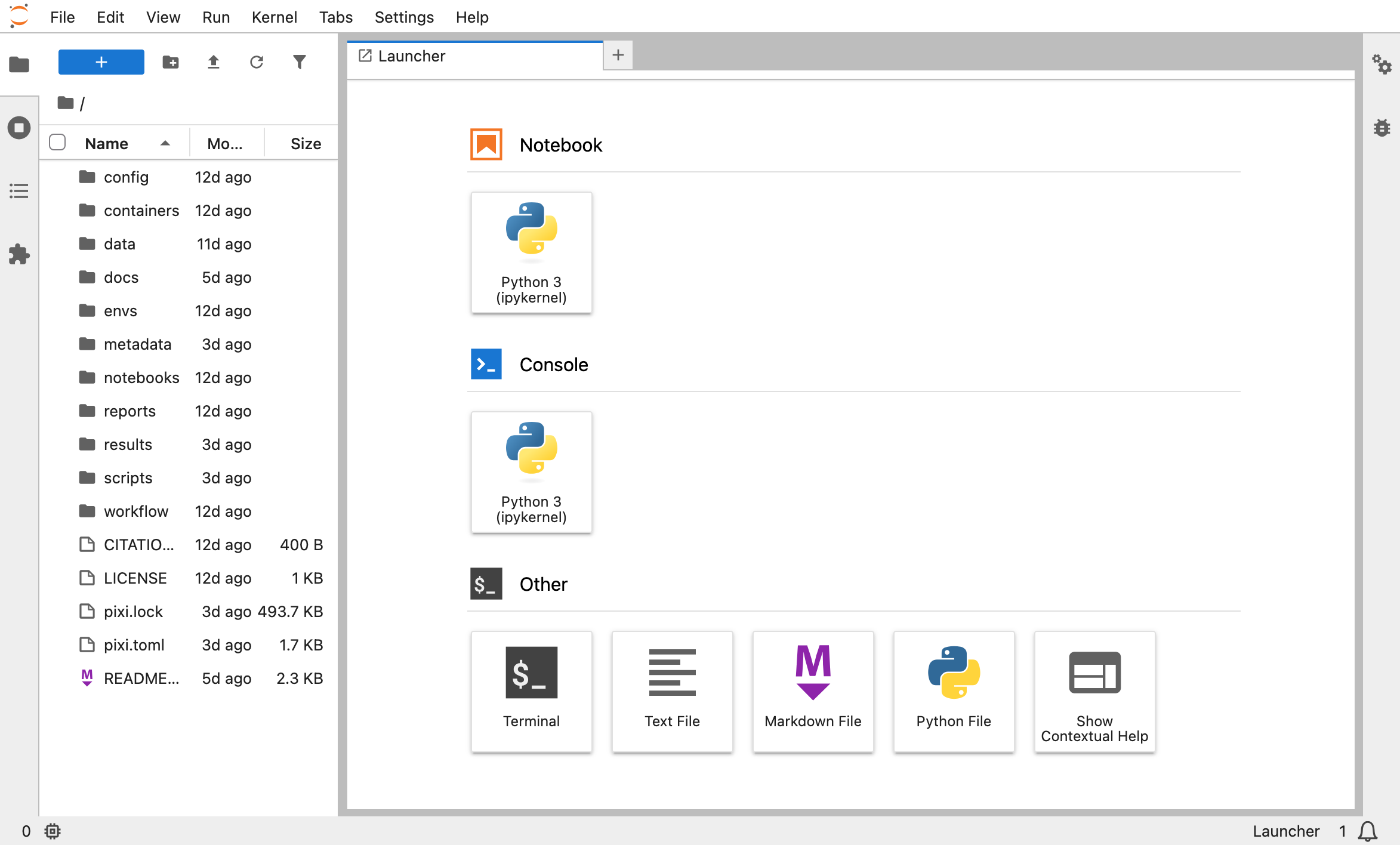
The terminal is now busy running Jupyter. Open a second terminal for other commands, and stop Jupyter with Ctrl-C (twice) when you are done.
2. Your first notebook
In JupyterLab’s file browser, open the notebooks/ folder, then File → New → Notebook and choose the Python 3 (ipykernel) kernel. Rename it to explore-reads.ipynb (right-click the tab → Rename).
A notebook is a list of cells. Markdown cells hold text; code cells hold code and, after you run them (Shift-Enter), their output.
Type each block below into its own cell and run it.
Cell 1 (Markdown):
# Exploring the LTEE reads

Questions: how long are the reads, and how does GC content vary between reads?
Exploration only: results that matter go into `reports/ltee-report.qmd`.
Cell 2 (code): go to the project folder and load the samples. The notebook’s kernel starts in notebooks/. To keep the rule that paths are relative to the project folder, the first code cell moves there:
# Run from the project folder, like the scripts (lesson 02).
import os
from pathlib import Path

if Path.cwd().name == "notebooks":
    os.chdir("..")

import matplotlib.pyplot as plt
import pandas as pd

samples = pd.read_csv("metadata/samples.tsv", sep="\t")
samples
The last expression of a cell (samples) is displayed as a table.
Cell 3 (code): one row per read.
# One row per read: sample, read length and GC content (first 5,000 reads of read 1).
# A FASTQ file has four lines per read; the second one is the sequence.
rows = []
for _, s in samples.iterrows():
    with open(s["fastq_1"]) as fh:
        for i, line in enumerate(fh):
            if i == 4 * 5000:
                break
            if i % 4 == 1:
                seq = line.strip()
                gc = 100 * (seq.count("G") + seq.count("C")) / len(seq)
                rows.append({"sample": s["sample"], "length": len(seq), "gc": gc})
reads = pd.DataFrame(rows)
reads.groupby("sample")[["length", "gc"]].describe().round(1)
A loop in a cell is fine for exploring. When the report in lesson 07 needs the same numbers, this code moves into a function in scripts/, where it can be reused and tested.
Cell 4 (code): a histogram. The #| lines are ignored by Jupyter but used by Quarto when it renders the notebook (lesson 07), which adds the caption and the alt text that Jupyter cannot add by itself:
#| label: fig-lengths
#| fig-cap: "Read length after trimming, first 5,000 reads of read 1 of each sample."
#| fig-alt: "Histogram of read lengths from 25 to 150 bases. A single tall bar at 150 bases holds about 60 percent of the reads; the rest are spread thinly between 25 and 149 bases."
fig, ax = plt.subplots(figsize=(6, 3))
ax.hist(reads["length"], bins=50, color="#2a78d6")
ax.set_xlabel("Read length (bases)")
ax.set_ylabel("Reads")
plt.show()
Cell 5 (Markdown): what you see.
About 60% of the reads are 150 bases long, the length of the sequencing run.
Trimming shortened the others, down to 25 bases, the shortest length that was kept.
Cell 6 (code): a quick number.
# Share of reads shorter than 100 bases, per sample
(reads.assign(short=reads["length"] < 100)
      .groupby("sample")["short"].mean()
      .mul(100).round(1)
      .rename("% reads < 100 bases"))
sample
SRR2584863 21.0
SRR2584866 21.8
SRR2589044 21.4
Name: % reads < 100 bases, dtype: float64Save the notebook (Ctrl-S / Cmd-S).
Save this as notebooks/explore-reads.ipynb (it is plain JSON; the outputs are empty):
notebooks/explore-reads.ipynb
{
 "cells": [
  {
   "cell_type": "markdown",
   "id": "66ca769b",
   "metadata": {},
   "source": [
    "# Exploring the LTEE reads\n",
    "\n",
    "Questions: how long are the reads, and how does GC content vary between reads? Exploration only: results that matter go into `reports/ltee-report.qmd`."
   ]
  },
  {
   "cell_type": "code",
   "execution_count": null,
   "id": "6ee60c5f",
   "metadata": {},
   "outputs": [],
   "source": [
    "# Run from the project folder, like the scripts (lesson 02).\n",
    "import os\n",
    "from pathlib import Path\n",
    "\n",
    "if Path.cwd().name == \"notebooks\":\n",
    "    os.chdir(\"..\")\n",
    "\n",
    "import matplotlib.pyplot as plt\n",
    "import pandas as pd\n",
    "\n",
    "samples = pd.read_csv(\"metadata/samples.tsv\", sep=\"\\t\")\n",
    "samples"
   ]
  },
  {
   "cell_type": "code",
   "execution_count": null,
   "id": "4db95a94",
   "metadata": {},
   "outputs": [],
   "source": [
    "# One row per read: sample, read length and GC content (first 5,000 reads of read 1).\n",
    "# A FASTQ file has four lines per read; the second one is the sequence.\n",
    "rows = []\n",
    "for _, s in samples.iterrows():\n",
    "    with open(s[\"fastq_1\"]) as fh:\n",
    "        for i, line in enumerate(fh):\n",
    "            if i == 4 * 5000:\n",
    "                break\n",
    "            if i % 4 == 1:\n",
    "                seq = line.strip()\n",
    "                gc = 100 * (seq.count(\"G\") + seq.count(\"C\")) / len(seq)\n",
    "                rows.append({\"sample\": s[\"sample\"], \"length\": len(seq), \"gc\": gc})\n",
    "reads = pd.DataFrame(rows)\n",
    "reads.groupby(\"sample\")[[\"length\", \"gc\"]].describe().round(1)"
   ]
  },
  {
   "cell_type": "code",
   "execution_count": null,
   "id": "2f884626",
   "metadata": {},
   "outputs": [],
   "source": [
    "#| label: fig-lengths\n",
    "#| fig-cap: \"Read length after trimming, first 5,000 reads of read 1 of each sample.\"\n",
    "#| fig-alt: \"Histogram of read lengths from 25 to 150 bases. A single tall bar at 150 bases holds about 60 percent of the reads; the rest are spread thinly between 25 and 149 bases.\"\n",
    "fig, ax = plt.subplots(figsize=(6, 3))\n",
    "ax.hist(reads[\"length\"], bins=50, color=\"#2a78d6\")\n",
    "ax.set_xlabel(\"Read length (bases)\")\n",
    "ax.set_ylabel(\"Reads\")\n",
    "plt.show()"
   ]
  },
  {
   "cell_type": "markdown",
   "id": "4f891436",
   "metadata": {},
   "source": [
    "About 60% of the reads are 150 bases long, the length of the sequencing run. Trimming shortened the others, down to 25 bases, the shortest length that was kept."
   ]
  },
  {
   "cell_type": "code",
   "execution_count": null,
   "id": "8007f1f0",
   "metadata": {},
   "outputs": [],
   "source": [
    "# Share of reads shorter than 100 bases, per sample\n",
    "(reads.assign(short=reads[\"length\"] < 100)\n",
    "      .groupby(\"sample\")[\"short\"].mean()\n",
    "      .mul(100).round(1)\n",
    "      .rename(\"% reads < 100 bases\"))"
   ]
  }
 ],
 "metadata": {
  "kernelspec": {
   "display_name": "Python 3 (ipykernel)",
   "language": "python",
   "name": "python3"
  },
  "language_info": {
   "name": "python"
  }
 },
 "nbformat": 4,
 "nbformat_minor": 5
}
3. Does it run without you?
In JupyterLab, Kernel → Restart Kernel and Run All Cells. If every cell runs without an error, the notebook does not depend on anything you did by hand. Do this before you share any notebook.
The same check from the command line, with a fresh kernel and no clicking, also writes an HTML copy of the result. In a second terminal:
cd ~/cbio7501/ltee-project
pixi run jupyter nbconvert --execute --to html notebooks/explore-reads.ipynb
[NbConvertApp] WARNING | Alternative text is missing on 1 image(s).
[NbConvertApp] Writing 305957 bytes to notebooks/explore-reads.htmlRead the warning: the histogram has no alt text in plain Jupyter output. Quarto reads the #| fig-alt line and fixes that (lesson 07).
4. Notebook, script or report?
A rule of thumb for this course: explore in a notebook, move code you reuse into scripts/, and put results you report into the Quarto report. Notebooks are fine to share as a record of exploration, as long as they run from top to bottom.
Break it: cells run out of order
Create a notebook in JupyterLab with these three cells, in this order:
lengths = [150, 98, 150, 25]print(sum(length >= min_length for length in lengths), "of", len(lengths), "reads kept")min_length = 100Now run cell 1, then cell 3, then cell 2. It works: 2 of 4 reads kept. Save the notebook as notebooks/out-of-order.ipynb. Everything looks fine.
notebooks/out-of-order.ipynb
{
 "cells": [
  {"cell_type": "code", "execution_count": 1, "id": "a1", "metadata": {}, "outputs": [],
   "source": ["lengths = [150, 98, 150, 25]"]},
  {"cell_type": "code", "execution_count": 3, "id": "a2", "metadata": {},
   "outputs": [{"name": "stdout", "output_type": "stream", "text": ["2 of 4 reads kept\n"]}],
   "source": ["print(sum(length >= min_length for length in lengths), \"of\", len(lengths), \"reads kept\")"]},
  {"cell_type": "code", "execution_count": 2, "id": "a3", "metadata": {}, "outputs": [],
   "source": ["min_length = 100"]}
 ],
 "metadata": {"kernelspec": {"display_name": "Python 3 (ipykernel)", "language": "python", "name": "python3"},
              "language_info": {"name": "python"}},
 "nbformat": 4, "nbformat_minor": 5
}
Look at the execution counts in the saved notebook: [1], [3], [2]. That is the clue. Now let a fresh kernel run it from top to bottom. Predict first:
pixi run jupyter nbconvert --execute --to html notebooks/out-of-order.ipynbNameError: name 'min_length' is not definedThe saved notebook shows the output 2 of 4 reads kept, but it cannot produce it. Anyone who reruns it gets an error. Fix it by moving the min_length cell above the cell that uses it, check again with nbconvert --execute, then delete the notebook:
rm -f notebooks/out-of-order.ipynb notebooks/out-of-order.htmlTroubleshooting
| Problem | What to do |
|---|---|
jupyter: command not found |
Start it with pixi run jupyter lab from the project folder. |
| JupyterLab opens but the browser shows nothing | Copy the full http://localhost:8888/lab?token=... link from the terminal. In WSL2, open it in your Windows browser. |
FileNotFoundError: ... 'metadata/samples.tsv' |
The first code cell did not move to the project folder: check that it runs os.chdir("..") and that the notebook is in notebooks/. |
No module named 'pandas' in JupyterLab |
The notebook uses a kernel from another Python. Choose Kernel → Change Kernel → Python 3 (ipykernel) and make sure you started Jupyter with pixi run. |
Port 8888 is already in use |
Another Jupyter is running; Jupyter picks the next port automatically. Use the link it prints. |
| The notebook file is several MB | It contains outputs: clear them (step 5). |
Apply it to your own project
Explore your own data in notebooks/ of your capstone project: load it, look at its size and a few summaries, make one quick plot. Then run it with jupyter nbconvert --execute and clear its outputs. Note what you want to keep: in lesson 07, results go into a Quarto report and code you reuse into scripts/.
Key points
- Start JupyterLab with
pixi run jupyter lab, so notebooks use the project’s environment. - Explore in notebooks; move reusable code into
scripts/and reported results into a Quarto report. - “Restart and run all” (or
nbconvert --execute) is the test that a notebook does not depend on your clicks. - Clear outputs before sharing or committing a notebook.
- Execution counts out of order (
[1] [3] [2]) are a warning sign.
Further reading
- Cheat sheet: Jupyter, with links to the official cheat sheets and references.
- JupyterLab documentation: https://jupyterlab.readthedocs.io/
- nbdime, diffs and merges for notebooks: https://nbdime.readthedocs.io/
- NBIS, Working with Jupyter (magics, widgets, nbdime for notebook diffs, nbval for testing notebooks): https://nbisweden.github.io/workshop-reproducible-research/pages/jupyter.html
- Quarto with Jupyter notebooks: https://quarto.org/docs/tools/jupyter-lab.html
- Rule A, Birmingham A, Zuniga C, et al. (2019). Ten simple rules for writing and sharing computational analyses in Jupyter Notebooks. PLoS Comput Biol 15:e1007007. https://doi.org/10.1371/journal.pcbi.1007007